Writing on the blog about some of the technical stuff I usually enjoy and/or work with is something that’s always in my plans but I never find the right time do it. Due to all this quarantine related stuff, both my sleeping habits and the kid’s are being somehow affected and, well, here I am, staring at a blank page trying to start writing about databases. And, well, since I don’t longer work for an international company I thought it would be a good idea to somehow practice my poor English skills.

This time my plan is to write about InfluxDB, a columnar oriented time-series database written in Go, and provide a quick tour of some of the most important characteristics of their storage engine.

I have been dealing with InfluxDB for a while and I have gone way deeper than I would like to quite a few times but I am by no means an expert, so, please, if I say something that’s not completely accurate, forgive me, and please, correct me.

I’ve dealt with both the OpenSource and the Enterprise versions but everything here is going to be based on the former (to the best of my knowledge the storage engine is the same in both alternatives). The details included later in the post are based on the 1.8.x and 1.7.x branches (I know the 2.0 introduces quite a lot changes but I won’t talk about them here).

Before getting started

Influx has gone through different storage engines through its short lifetime: LevelDB, BoltDB (not sure if there’s anymore) and, and this is just an educated guess, any of them completely satisfied the requirements that the InfluxDB folks were looking for: large batch deletes, hot backups, high throughput or a good compression performance among many others. So, in order to solve the previous points (it’s not an exhaustive list), they decided to go on their own and write a new storage engine (it’s a brave bet).

Everything I am going to write about here is focused on this storage engine and I have no experience with the Influx versions where the underlying storage engine was LevelDB or BoltDB.

InfluxDB concepts

Before we go into the details of the storage engine let me introduce a few concepts I think all of us should know about.

Everything starts with a database concept, similar to a traditional RDBMS, which acts as the container of many of the capabilities that Influx provides: user management, retention policies, continuous queries, … Everything related to a database is represented under a folder in the filesystem.

A retention policy describes how long the data is kept around and how many copies of this data are stored in the cluster (for the OpenSource version the replication setting has no effect).

Measurements are the “data structure” used to model how the data is stored in Influx and the fields associated with it.

Fields represent the actual data value. These are required and, something really important, they are not indexed.

Tags represents metadata associated with the aforementioned fields. They are optional, but they are very useful because they are indexed and allow you to perform group by and/or filter operations (you can filter on fields as well, but since they are not indexed, this is not a performant operation).

Series are a logical grouping of data defined by a measurement, a set of tags and a field. To me, this is one of the most important concepts that need to be clear while working with InfluxDB, because many of the different concepts revolve around it.

Shards contains the actual encoded and compressed data. They are represented by a TSM file on disk (more on this later). Every shard contains a specific set of series so all the points falling on a given series will be stored in the same shard.

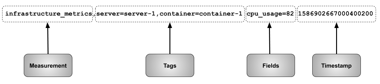
In order to get your data points inserted into the database, Influx defines a text-based protocol named line protocol.

An example of how a single data point looks like in the line protocol and how it maps to the concepts described before is shown in the picture below:

InfluxDB storage engine

At the beginning of the post, I described some of the features that, per my understanding, the Influx folks were looking for when building their storage engine and how all these requirements led them to their current storage solution.

Their storage solution is similar to an LSM Tree and, from a high-level perspective, it is composed by:

• A write-ahead log
• A collection of TSM (read-only) files where the actual time series data is stored (similar to the SSTables)
• TSI files that serve as the inverted index used to quickly access the information. Prior to this version of the index, the data was held into an in-memory data structure, making it difficult to support high-cardinality scenarios (millions of series).

Before we move forward, a short note about how I plan to organize the contents. The original idea was to put everything I wanted to write down into a single post but it would be probably a little bit dense so I have decided to split it into 3 different parts:

• The current one with the introduction to Influx, the overview of the storage engine and a quick tour around the WAL component and its cache counterpart.
• The second one will cover the details about the TSM.
• The third one will cover details about the TSI.

For this post, let’s try to go a little bit deeper into the write ahead log (WAL) and its cache counterpart.

Write ahead log (WAL)

The WAL is a write-optimized data structure that allows the writes to be durable and its main goal is to allow the writes to be appended as fast as possible so it is not easily queryable.

When a new write comes into the system the new points are:

• Stored at an in-memory cache (more about this in the next section).
• Serialized, compressed using Snappy and written to the WAL.

If we take a look at the source code we can see where this actually happens:

// WritePoints writes metadata and point data into the engine.
// It returns an error if new points are added to an existing key.
func (e *Engine) WritePoints(points []models.Point) error {
    ….
    // first try to write to the cache
    if err := e.Cache.WriteMulti(values); err != nil {
        return err
    }
 
    if e.WALEnabled {
        if _, err := e.WAL.WriteMulti(values); err != nil {
            return err
        }
    }
    return seriesErr
}

Note that we could disable the WAL and, in this case, writes will only exist in the cache and could be lost if a cache snapshot has not happened.

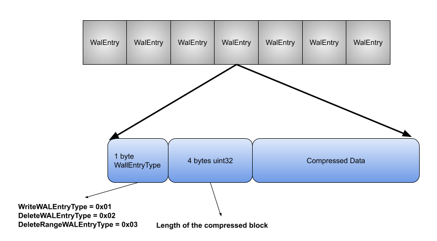
The format used to describe every one of the entries appended to the WAL follows a type-length-value encoding scheme with a single byte representing the type of the entry being stored (write, delete or a range delete), a 4 byte uint32 representing the length of the compressed block, followed by the actual compressed data block.

Looking again at the source code here we can see how the actual writing is performed:

// Write writes entryType and the buffer containing compressed entry data.
func (w *WALSegmentWriter) Write(entryType WalEntryType, compressed []byte) error {
    var buf [5]byte
    buf[0] = byte(entryType)
    binary.BigEndian.PutUint32(buf[1:5], uint32(len(compressed)))
 
    if _, err := w.bw.Write(buf[:]); err != nil {
        return err
    }
 
    if _, err := w.bw.Write(compressed); err != nil {
        return err
    }
 
    w.size += len(buf) + len(compressed)
 
    return nil
}

Cache

The cache component is an in-memory data structure that holds a copy of all the points persisted in the WAL. As we’ve already mentioned in the previous section, when a new write comes into the system the new points are stored in this cache.

The aforementioned points are indexed by the key which is formed by the measurement name, the tag set and the unique field key. If we go back to our previous example where we had a single write coming into the system:

infrastructure_metrics,server=server-1,container=container-1 cpu_usage=82

The key would be represented by something like this:

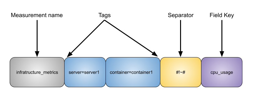
The points stored in the cache are not compressed and an upper bound can be set so we can prevent unexpected out of memory situations (if the upper bound limit is exceeded new writes coming into the system will be rejected) and prevent the database service to be unexpectedly restarted.

When the number of elements in the cache reaches a certain lower bound (it’s configurable as well) a snapshot of the cache is triggered to a TSM file and the corresponding WAL segment files are removed.

If we take a quick look to the source code we can see the behavior described in the previous paragraph:

// compactCache continually checks if the WAL cache should be written to disk.
func (e *Engine) compactCache() {
    t := time.NewTicker(time.Second)
    defer t.Stop()
    for {
        e.mu.RLock()
        quit := e.snapDone
        e.mu.RUnlock()
 
        select {
        case <-quit:
            return
 
        case <-t.C:
            e.Cache.UpdateAge()
            if e.ShouldCompactCache(time.Now()) {
                start := time.Now()
                e.traceLogger.Info("Compacting cache", zap.String("path", e.path))
                err := e.WriteSnapshot()
                if err != nil && err != errCompactionsDisabled {
                    e.logger.Info("Error writing snapshot", zap.Error(err))
                    atomic.AddInt64(&e.stats.CacheCompactionErrors, 1)
                } else {
                    atomic.AddInt64(&e.stats.CacheCompactions, 1)
                }
                atomic.AddInt64(&e.stats.CacheCompactionDuration, time.Since(start).Nanoseconds())
            }
        }
    }
}

When a new read operation is received, the storage engine will merge data from the TSM files with the data stored in the cache (so you can read data that hasn’t been snapshotted into the TSM files yet). At query processing time, a copy of the data is done so any new write coming into the system won’t affect the results of any running query.

Conclusion

This post has been a short intro to InfluxDB and a brief overview of its storage subsystem. In addition to the previous intros, we’ve covered a few details of the WAL + Cache storage subsystem elements. As I have already mentioned, my idea is to publish two more posts: one of them covering a few details of the TSM part and the other one going through the inner workings of the TSI component.

Of course, I am aware this is just an introduction, and the devil is in the details, but I do hope this provides you some insights into a few database design concepts and how a concrete database applies them.

Thanks for reading.